
Thank you for visiting this site. This article covers “Simpson’s Paradox.”
The world of data hides a frightening trap. Divide a population into two groups and compare them, and A may look superior. Aggregate all the data together and B comes out on top. What holds within each subgroup need not hold in the combined total. This is Simpson’s Paradox.
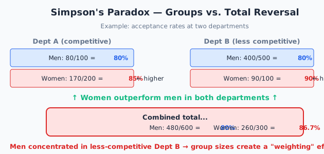
A Concrete Example
Suppose a university is accused of gender bias in admissions.
Engineering School
- Men: 800 applicants, 480 admitted (60% acceptance rate)
- Women: 100 applicants, 70 admitted (70% acceptance rate)
Liberal Arts School
- Men: 200 applicants, 40 admitted (20% acceptance rate)
- Women: 900 applicants, 270 admitted (30% acceptance rate)
Looking at each school individually: women have a higher acceptance rate in both schools.
But combine all applicants:
- All men: 1,000 applicants, 520 admitted (52% acceptance rate)
- All women: 1,000 applicants, 340 admitted (34% acceptance rate)
Wait — men have a higher overall acceptance rate!
Women outperform men in every individual school, yet men lead overall. The numbers do not lie; the conclusion simply reverses. This is Simpson’s Paradox.
Why the Reversal Happens
The key is the distribution of applicants across schools.
In this example, men apply predominantly to the higher-acceptance Engineering School (800 applicants), while women apply predominantly to the lower-acceptance Liberal Arts School (900 applicants).
Men concentrate in the easier school; women concentrate in the harder school. Even though women outperform within each school, the overall acceptance rate is heavily influenced by which school each group applies to.
The hidden third variable (in this case, choice of school) is called a confounding variable. Ignore the confounding variable and aggregate naively, and Simpson’s Paradox appears.
A Real Historical Case
This is not a desk-bound abstraction. Simpson’s Paradox has caused real-world confusion.
In 1973, the overall admission rate at UC Berkeley was 44% for men and 35% for women, raising suspicions of gender discrimination. But a department-by-department analysis found that in most departments women’s admission rates equaled or exceeded men’s.
The explanation: women disproportionately applied to highly competitive departments with low acceptance rates. This real example is now a standard illustration in statistics textbooks.
Lessons for Data Analysis
The most important lesson Simpson’s Paradox teaches: the conclusion can change depending on which level of aggregation you examine.
Looking only at overall figures can lead to conclusions that are the exact opposite of the truth. But subdividing too finely produces sample sizes too small for statistical reliability.
The key habit is always asking: “Is there a hidden confounding variable in this data?” Blindly trusting simple aggregate statistics is especially dangerous in business decision-making and policy.
In medicine, Simpson’s Paradox frequently arises when evaluating treatments. If severe and mild patients are assigned to treatments in unequal proportions, the combined analysis can make a good treatment look bad. This is one reason why randomized controlled trials (RCTs) are the gold standard in medical research: randomization balances confounders across groups.
Split the groups, or combine them?
The most troublesome thing about Simpson’s paradox is that whether splitting or combining is correct cannot be decided from the data alone.
The same set of numbers yields two conclusions: split them and A wins, combine them and B wins. Both are arithmetically correct, so statistics on its own cannot settle it.
What settles it is the causal order.
| Where the splitting variable sits | Example | Which result to read |
|---|---|---|
| Before the treatment | patient age, severity of illness | the split result |
| After the treatment | a side effect caused by the treatment | the combined result |
| Unrelated to the treatment | the patient’s ID number | makes no difference either way |
When judging a treatment’s effect, a patient’s severity is fixed before treatment begins. Severe cases get assigned the stronger treatment, so comparing without splitting makes the stronger treatment look worse. Here splitting is right.
Split on a side effect produced by the treatment, on the other hand, and you are cancelling out part of the very effect you are measuring. Here you must not split.
A case that went to court
The famous one is the 1973 graduate admissions data from Berkeley.
Overall, 44 percent of men were admitted against 35 percent of women, and the university was suspected of sex discrimination. Broken down by department, though, women had the higher admission rate in most departments.
The trick lay in where people applied. Women applied in larger numbers to competitive departments with low admission rates, men to departments with high ones.
- Overall: men appear to be favoured
- By department: women are slightly favoured
- What was actually happening: selection within departments was not skewed; the distribution of applications was
Here the department is chosen by the applicant at the point of applying, so it sits before the treatment, which makes the split view the one closer to reality.
Staring at the numbers will not tell you which is right. You have to work out “what is affecting what” first. I make a point of settling that order before starting an analysis.
How it got its name
Simpson’s name is attached, and he was not the first to point the phenomenon out.
- Karl Pearson (1899) reported cases where mixing populations changes the correlation
- Yule (1903) set out the same phenomenon in contingency tables
- Edward Simpson (1951) treated it systematically in a paper, and the name stuck
- Colin Blyth (1972) popularised the label “Simpson’s paradox”
For that reason it is sometimes called the Yule–Simpson effect.
Simpson himself did not call it a paradox, since nothing mathematically contradictory occurs. His position was that the arithmetic is entirely correct and the only thing surprised is human intuition.
Even after the name settled, some statisticians prefer the neutral term reversal.
The trap in averaging averages
Mathematically, the phenomenon comes from adding together averages that carry different weights.
When the denominators differ between groups, the overall ratio is dragged toward the larger group. You can be ahead within every group and still lose overall, if the groups where you are ahead hold few people.
Ratios cannot be added or averaged. That is the basic caution.
- Correct: add the numerators and the denominators, then divide
- Never do this: take a plain average of each group’s ratio
- When comparing: either equalise the group sizes or keep the groups separate
Batting averages, utilisation rates, completion rates. With any metric whose denominator moves, simply keeping this in mind heads off a great many accidents.
Related paradoxes that defy probabilistic intuition
Related paradoxes where the arithmetic is correct and the answer refuses to sit with intuition.




Summary
This article covered “Simpson’s Paradox.”
Statistics is a powerful tool when used correctly, but can become a weapon for disinformation when misused. Whenever you read data, the habit of pausing to ask “is this the right way to aggregate?” is worth cultivating — and this paradox shows exactly why.
To return to the full list of paradoxes, follow the link below.
Thank you for reading. We hope to see you in the next article.

Also popular with readers
📚 Series: The World's Paradoxes (32/81)