
Thank you for visiting this site. This article covers the “Inspection Paradox.”
Suppose you turn up without checking the timetable at a stop where buses run every 10 minutes on average. Straightforwardly you would expect to wait about 5 minutes, and in practice you wait considerably longer. The buses are not late and you are not unlucky. There is a mechanism that puts a bias into the measurement itself, and it shows up in the same shape all over ordinary life.
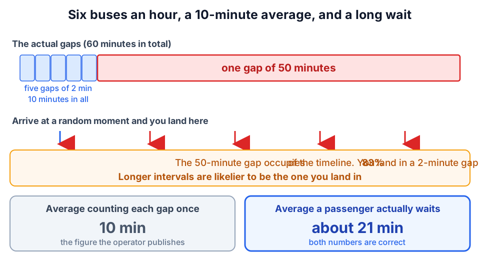
Waiting for a bus that averages 10 minutes
Let me check with a simple example.
Say six buses arrive in an hour. That averages 10 minutes apart, but the intervals are not exactly even; there is spread.
Suppose in one hour the gaps run 2, 2, 2, 2, 2 and 50 minutes. Sixty minutes in total, averaging 10.
Now arrive at a random time without consulting the timetable. Ask which gap you land in.
There are five 2-minute gaps, and together they add up to only 10 minutes. The single 50-minute gap occupies 50 minutes of the hour.
Arriving at random, you land in the 50-minute gap with about 83% probability. You rarely hit a short gap.
Work out the average wait and it comes to roughly 21 minutes. A bus every 10 minutes, and you wait more than twice that.
Longer intervals are easier to hit
The trick lies in how the interval gets selected.
Count the gaps one by one, equally, and the average really is 10 minutes. The moment you select by “arriving at a random time,” the gaps stop being equal.
A longer gap occupies more area on the time axis, so you are more likely to land in it. The 50-minute gap is 25 times easier to hit than a 2-minute one.
The structure is exactly that of the friendship paradox. There, the bias was “people with more friends appear on more people’s friend lists.” Here it is “longer intervals are more likely to be selected as the one you land in.”
Both are cases of being chosen in proportion to size, known as size-biased sampling.
If the service ran on perfectly even intervals with no spread at all, the effect would vanish. The greater the spread, the longer the perceived wait.
The wait is decided by the spread alone
The example above was extreme, but the wait can be computed directly from the variability of the service.
The formula with spread included
With mean interval m and interval variance v, the mean wait is:
(v + m×m) / (2×m)
With zero spread this is m/2, half the mean interval. Run exactly to timetable and the straightforward “half” answer is correct.
For a 10-minute mean interval, varying only the spread:
| State of the service | Variance | Mean wait |
|---|---|---|
| Perfectly even | 0 | 5.0 min |
| Somewhat variable | 25 | 6.3 min |
| Completely random | 100 | 10.0 min |
| Extremely skewed (five 2s and a 50) | 320 | 21.0 min |
Random arrivals mean waiting a whole interval
Note the third row. If bus arrivals are completely random — each independent of the last — the mean wait is exactly the mean interval, 10 minutes.
Not half, but the whole thing. And however long you have already waited, you still face another 10 minutes on average. Twenty minutes in, your expected remaining wait has not fallen.
This is the memoryless property, and it appears wherever mutually independent events pile up: phone calls arriving, requests hitting a server. The feeling that “it must be due any moment” keeps being betrayed, and that is not your imagination.
University class sizes do the same thing
A more familiar example, often cited, is class size.
Suppose a university announces that “our average class has 30 students.” The figure is not a lie. Add up the students in every class, divide by the number of classes, and it really is 30.
Ask students “how many people are in the classes you take,” and a far larger number comes back.
Same reason. Two hundred people sit in the 200-person lecture, and five sit in the five-person seminar. Count by student and large classes get reported dozens of times more often.
The university’s number and the students’ experience are both correct. The only difference is “did you count classes, or count students?” It is the single most useful thing to notice when reading statistics.
Why perceptions of crowding are off
Once you see the structure, several everyday oddities explain themselves.
Roads are uncongested for far more hours than they are congested, and yet almost every driver experiences congestion. Naturally: there are more cars on the road during the congested hours.
Restaurants are the same. A venue may be quiet for more hours than it is busy, and yet most of the people who came as customers were there during the busy period.
Surveys of household size run high unless designed for. Households with more children put more people forward as respondents.
Nobody is lying in any of these. Different units of counting produce different numbers.
The trap for people designing surveys
What makes the bias awkward is that it walks in without malice. Common shapes:
- User surveys: frequent users have more chances to respond and dominate the aggregate
- Measuring queue times: ask people in the queue and long waiters are the ones you catch
- Average length of hospital stay: sample current inpatients and long stays are over-represented
- Equipment lifetime studies: sample working units and the short-lived ones are already broken and unsampled
- Customer tenure: sample current subscribers and everyone who cancelled quickly drops out
All share the feature of drawing the sample from “what exists right now.” The longer something has lasted, the likelier it is to exist at any given moment.
Three ways to avoid it
The remedies are not difficult.
First, declare up front what counts as one. Just writing whether you counted classes or students, occasions or people, prevents most reader confusion.
Second, track from a starting point. For length of stay, follow everybody from the day of admission and the bias disappears. Statistics calls this a cohort study.
Third, where it is unavoidable, correct with weights. If you know longer intervals are more likely to be chosen, reweight in inverse proportion to length and you recover the original distribution.
None of these is a specialist technique. The habit of first asking “where was this number taken from?” prevents most of it.
Where the name comes from
The name inspection paradox comes from quality inspection and studies of equipment uptime.
To learn the mean time to failure of a machine, sampling machines that happen to be running at a given moment picks up only the “long-lived units.” Short-lived ones have already failed and have little chance of being selected.
Medicine knows the same problem. Sample current inpatients to find mean length of stay and long stays are over-represented, so the figure comes out too high.
The remedy is not hard: decide at the outset whether you are counting individuals or counting time and occasions, and state it. Since learning this distinction, whenever the word average appears I check first “what was counted as one?”
Related paradoxes that defy probabilistic intuition
Related paradoxes where the arithmetic is correct and the answer refuses to sit with intuition.




Summary
This article covered the “Inspection Paradox.”
Waiting 20 minutes for a bus every 10, and a class averaging 30 that feels like 100, both come down to quietly swapping the unit of counting midway. Both figures are correct; they are simply measuring different things.
The word average has a strong power to make you feel you understand, so this is a pitfall we will be living with for a long time.
To return to the full list of paradoxes, follow the link below.
Thank you for reading. We hope to see you in the next article.

Also popular with readers
📚 Series: The World's Paradoxes (29/81)